vSphere Performance - Telegraf, InfluxDB and Grafana 7 - Building Grafana Dashboards

Aug 6, 2020 (Last modified: Aug 6, 2020)vsphere grafana influx telegraf ·

Overview

Intro

This post will be all about how you can get started with building informative and beautiful dashboards of your vSphere environment with Grafana 7.

The vSphere performance data is pulled with the vSphere input plugin for Telegraf, and the data is stored in a InfluxDB database. This post will build on the work done in part 2 of this series, but if you already have a Influx database with vSphere data you should be able to follow along.

Ultimately the goal of this post (and upcoming ones) is to show how easy, and fun, it is to build Grafana dashboards so even if you have other datasources I think there should be some valid pointers for you as well.

There's a lot to discuss when it comes to Grafana so I'll split it in multiple posts. This first post will be about how to get started and the Graph panel. The next posts will be about Grouping, filtering and variables which is essential to dashboarding, and we will have some posts on different panel types.

I have written a few blog posts on creating Grafana dashboards previously. Some of these are not entirely about Grafana dashboards, but they include some tips on a few panels and visualizations

These are still valid, but I wanted to do a follow up by utilizing the new Grafana release and the new panel editor shipped in version 7.

Installing and configuring Grafana

For installing Grafana I will refer you to the documentation which is very good. It details the steps with examples for both Linux distros, Windows, macOS and Docker containers.

For the purpose of this blog post we do not have to change any of the default configuration either so we'll leave that for now. In an upcoming blog post we will check out how to secure some of the components in our Performance monitoring solution and then we'll revisit Grafana configuration.

With Grafana has been installed and running we should be able to start playing around with some data.

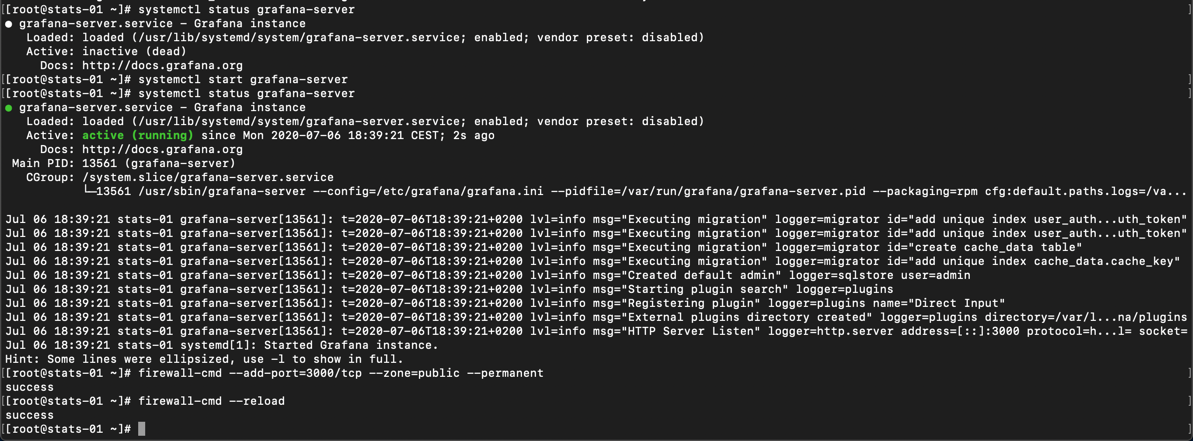
Remember that for the purpose of this blog post I'm using vSphere data collected by the Telegraf agent pushing to an InfluxDB database as discussed in this previous post

As I excpect most people will access Grafana with a browser running external to the Grafana server remember to open any firewalls between your client browser and the Grafana server (http/s port 3000 by default).

Adding a datasource

The first thing we'll do after logging in and changing the default password is to add a datasource. This is the connection between Grafana and the InfluxDB database.

For detailed steps please refer to the Grafana documentation. For the purpose of this blog post we'll add an InfluxDB datasource running on the same server as Grafana.

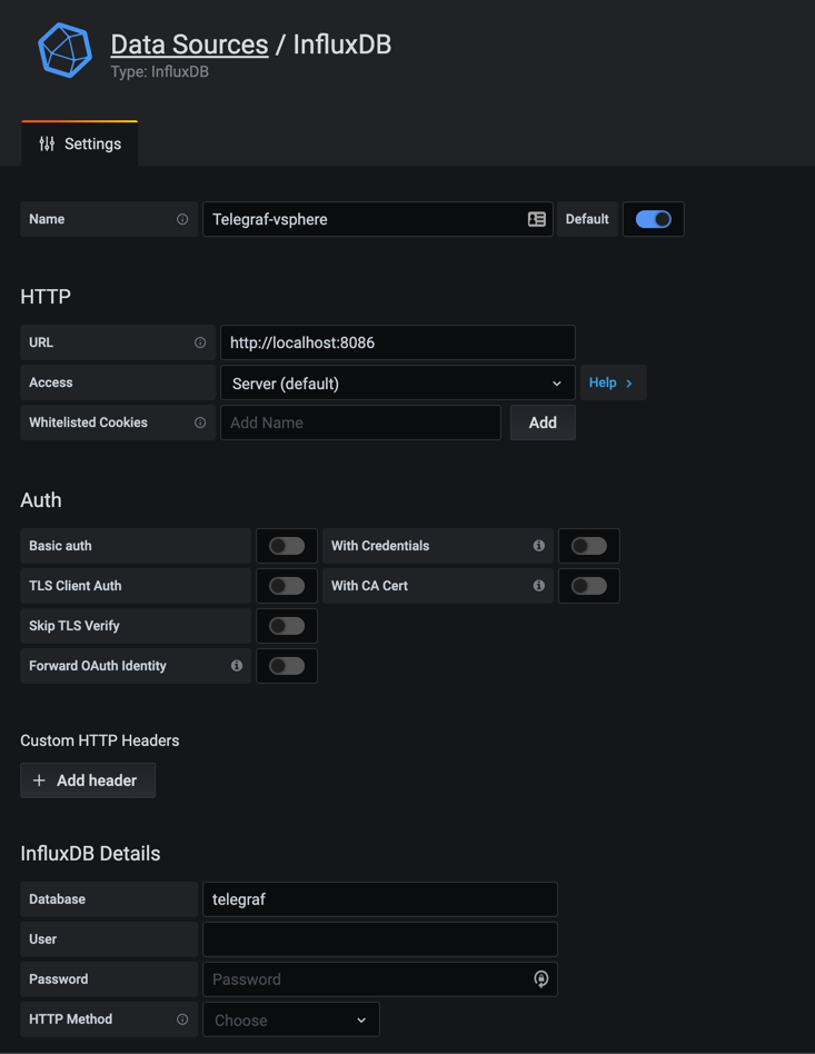
After you specify the address to the InfluxDB server (http://localhost:8086 in this example) and the name of the database (telegraf) we click "Save & Test" at the bottom of the page and should get a success message back.

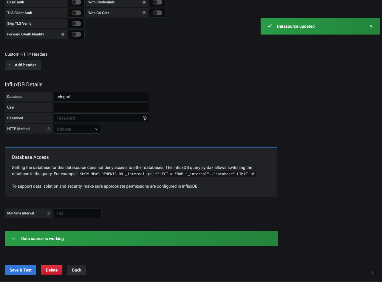
As this Telegraf datasource could contain more than vSphere data I'll leave the "Min time interval" setting empty. We will see how this affects our dashboard queries later on.

Get started with building dashboards

A note on importing dashboards

Grafana has the ability to import dashboards. Importing a finished dashboard can quickly give you some nice visualizations on top of your vSphere data. However I do encourage you to use this for inspiration only.

Let me give you a fair warning at this point: This blog series, and especially the Grafana parts, is quite lengthy. If you want to import some finished dashboards created for the vSphere data pulled by Telegraf check this page, if not read on and see how you easily can get started with building you own

I am a strong believer of that the true value comes when you build dashboards that is made for your environment and needs. You'll get better insight and understanding of your own data which I think is more complicated to get if using pre-built dashboards.

All environments are different, and there are many different usecases and focus points for dashboards. What is important for me in my environment isn't necessarily important for you in yours.

Maybe you have a traditional SAN solution and need to track utilization and performance of many different datastores while I use vSAN and have only one datastore.
A dashboard created for my small home lab might not be performant in a larger environment with many more objects and metrics.

These are just a few examples I've encountered when testing dashboards others have built and from feedback given by others.

Our first dashboard and the Graph panel

Well, it's not my first dashboard, and maybe not yours either. But it's the first for this series...

The first thing that greets us when creating a new dashboard is an empty canvas where we are asked to add a Panel. Panels are the different visualization "boxes" in a dashboard and can have different forms. From graphs, to singlestat, tables and gauges.

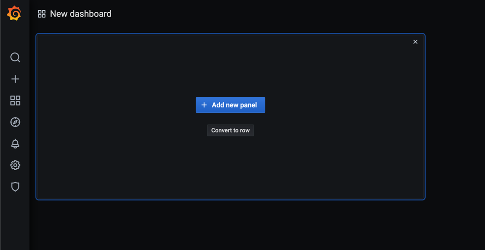
We'll start of by adding a few queries for Host CPU and Memory usage. For this we'll select the correct datasource and then click the "select measurement" field which will bring us a dropdown with our measurements (or tables if you will) in Influx.

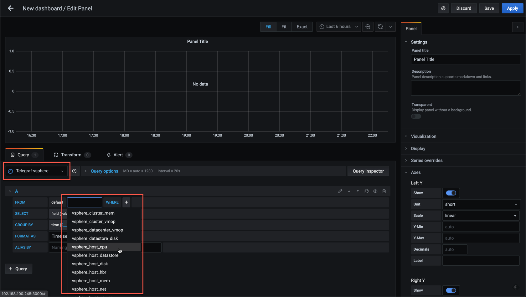
We'll select the vsphere_host_cpu measurement and then specify which of the cpu metrics we want to display. In Influx this is referred to as Fields, and for our first metric we'll select usage_average which contains the CPU usage in percentage and Grafana should start displaying a graph with your data. This data will be the average CPU usage for all hosts in your Telegraf database.

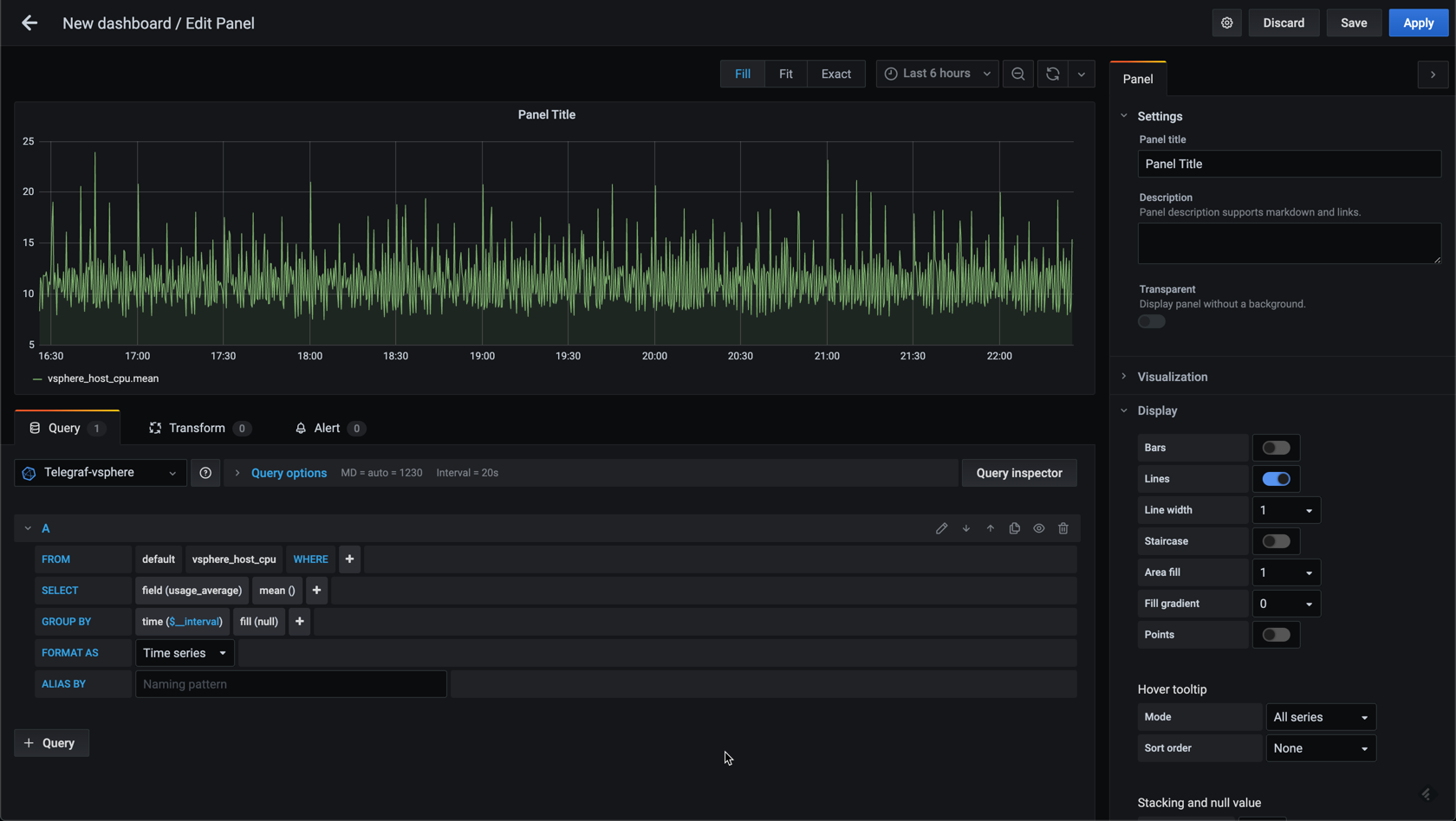
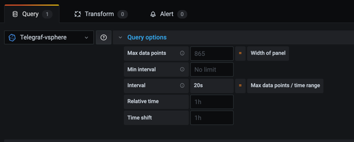
If you only see dots/points in the graph which is not connected we need to adjust the time grouping. Grafana tries to figure out the grouping based on the data, but sometimes you'll need (or want) to override this. This is done in the Query options part of the editor. Here you can specify a minimum time interval for your data (20 seconds for vSphere realtime data). Note that in my case the Interval already is correct, hence I can leave this as it is.

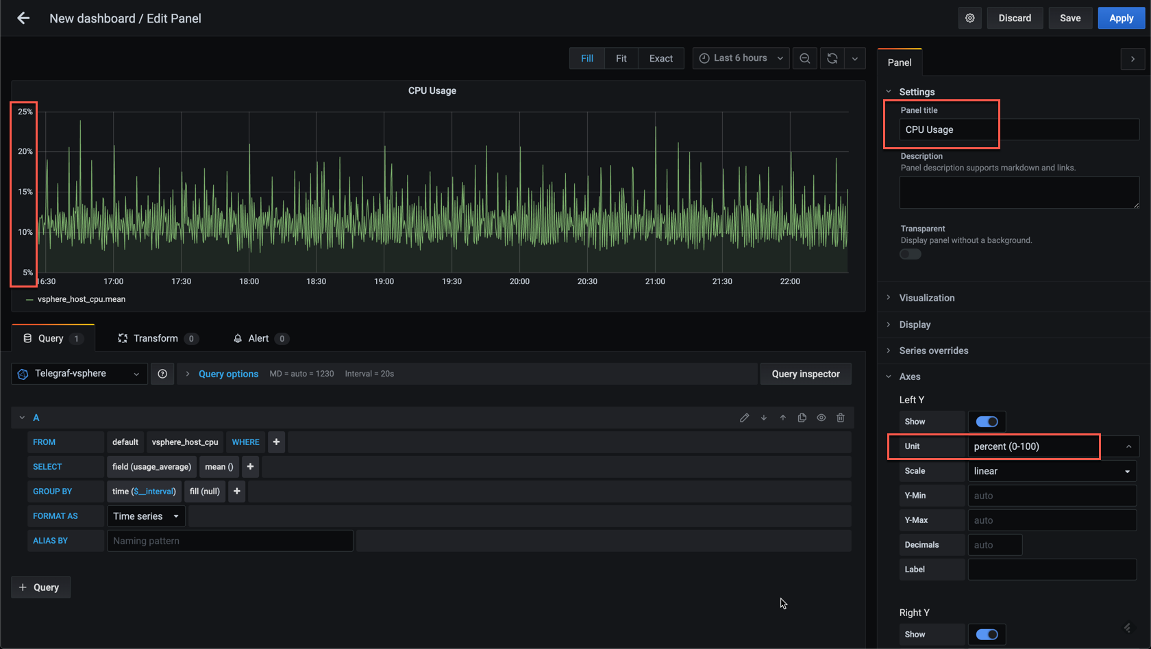
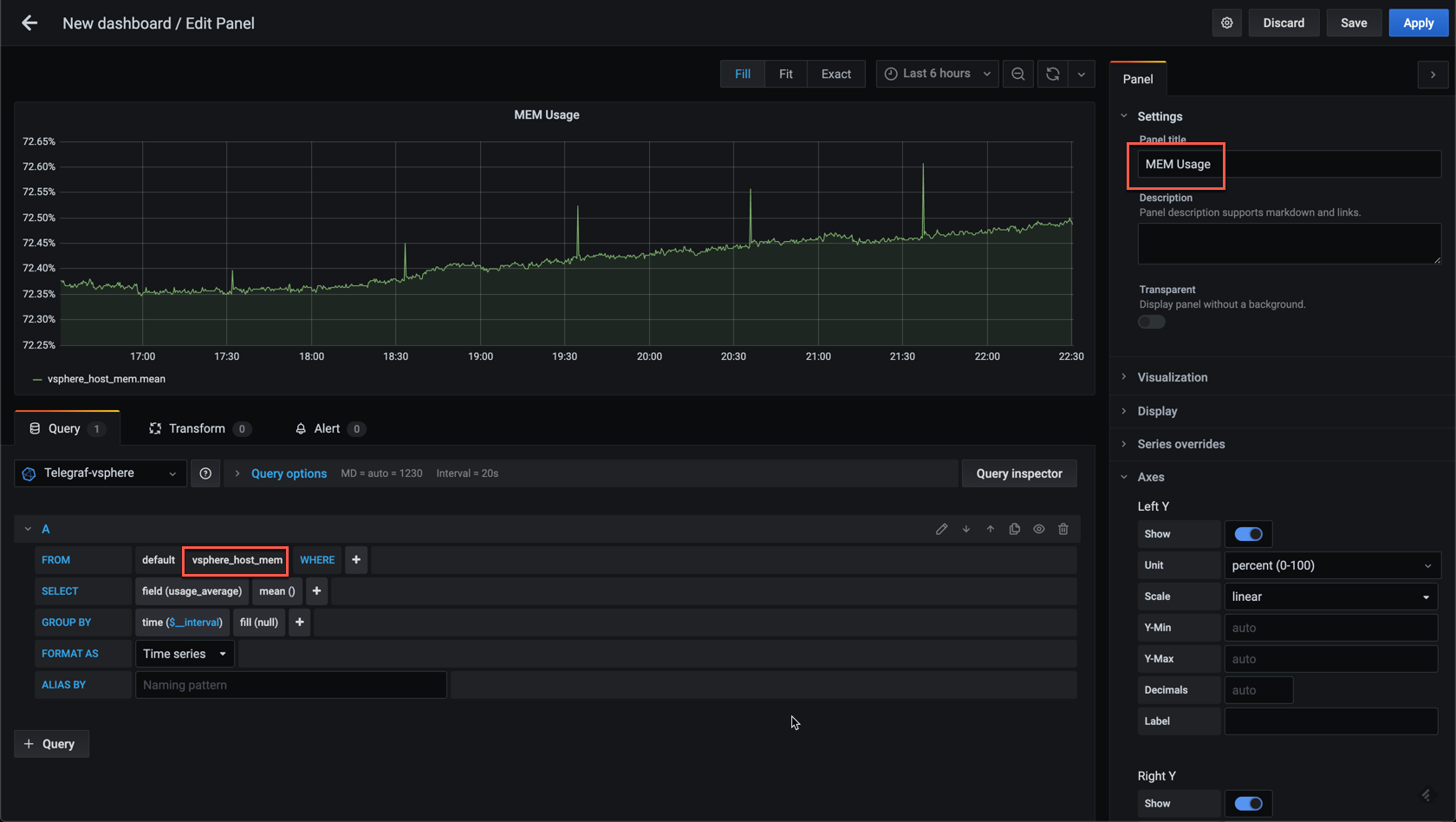
In the new Panel editor (changed in Grafana 7) on the right hand side we can add some specifics for our new panel. It's here you can tweak more of the visualization settings, like line width, graph fill, thresholds etc. For this first panel we'll leave the defaults, we'll just add a Title and the Unit for the data.

As a first panel I'm happy with this, but let's also add a similar graph for the memory. We can quickly do this by duplicating the CPU panel.

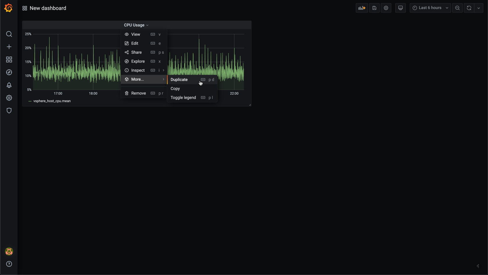
Now you should have two identical graph panels. Edit the second panel and update the metric to the vsphere_host_mem measurement, and update the title accordingly.

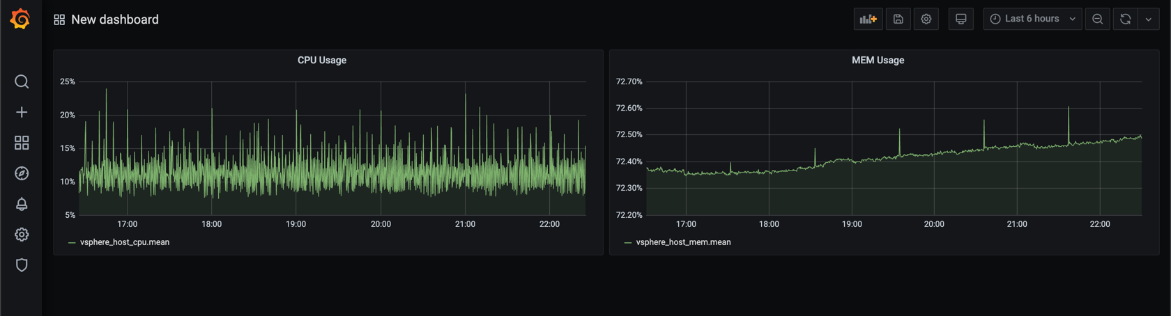
Voila! With just a few clicks we now have both the CPU and Memory usage for our hosts

Summary

There's lots more to discuss when it comes to creating dashboards, like the different panel types available, grouping, variables, dashboard linking, sharing etc, which we'll take a look at in upcoming posts.

Thanks for reading and reach out if you have any questions or comments.

This page was modified on August 6, 2020: Fixed title